RDBMS
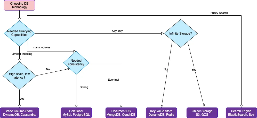
How to choose DB for your project based on query pattern?
Cheatsheet

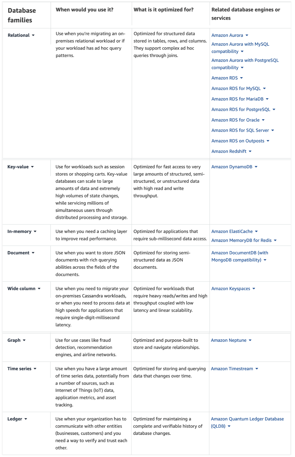
Database classification
| Database Family | Optimization Focus | Sample Query | Example Databases |
|---|---|---|---|
| Relational Databases | Structured data, complex queries, ACID compliance, data integrity, transaction support | SELECT * FROM customers WHERE age > 30; | MySQL, PostgreSQL, Oracle |
| Document Databases | Storing and retrieving JSON-like documents, flexible schema, horizontal scalability, denormalized data | db.customers.find({ age: { $gt: 30 } }); | MongoDB, Couchbase, Amazon DynamoDB |
| Key-Value Stores | Simple key-value data storage and retrieval, high throughput, eventual consistency, distributed caching | GET customer:12345; | Redis, Riak, Amazon DynamoDB |
| Column-Family Databases | Storing and querying large amounts of flexible data, high write performance, distributed design, append-only storage | SELECT * FROM customers WHERE city = ‘New York’; | Apache Cassandra, ScyllaDB, HBase |
| Graph Databases | Managing highly interconnected data and complex relationships, graph traversal, pattern matching, native graph processing | MATCH (p:Person)-[:FRIEND]->(f:Person) WHERE p.name = ‘John’ RETURN f.name; | Neo4j, Amazon Neptune, ArangoDB |
| Time-Series Databases | Storing and analyzing time-stamped data, optimized for time-series data, compression techniques, data retention policies | SELECT * FROM sensor_data WHERE time > ‘2023-01-01T00:00:00Z’; | InfluxDB, TimescaleDB, Prometheus |
| NewSQL Databases | Combining benefits of SQL with scalability of NoSQL, high availability, distributed transactions, automatic sharding | SELECT * FROM orders WHERE date > ‘2023-01-01’; | Google Spanner, CockroachDB, NuoDB |
| Object-Oriented Databases | Managing complex data types and relationships, object-oriented data modeling, support for complex data structures, rich querying capabilities | SELECT * FROM employees WHERE department = ‘Engineering’; | db4o, ObjectDB, Objectivity/DB |
| Multi-Model Databases | Supporting multiple data models within a single system, polyglot persistence, native multi-model query language, unified data access | FOR doc IN documents FILTER doc.status == ‘active’ RETURN doc; | ArangoDB, OrientDB, MarkLogic |
| Search Databases | Indexing and querying unstructured or semi-structured data, full-text search, relevance ranking, faceted search | GET /search?q=keyword; | Elasticsearch, Apache Solr, Splunk |
| Spatial Databases | Storing and querying spatial data, spatial indexing, spatial analysis functions | SELECT * FROM points WHERE ST_CONTAINS(area, point); | PostGIS, MongoDB (with GeoJSON), Oracle Spatial |
| In-Memory Databases | High-speed data retrieval and processing, caching, real-time analytics, low-latency applications | GET employee:12345; | Redis, Memcached, Apache Ignite |
| Content Databases | Managing and delivering digital content, metadata storage, content versioning, content distribution | SELECT * FROM articles WHERE category = ‘Technology’; | CouchDB, Amazon DocumentDB, eXist-db |
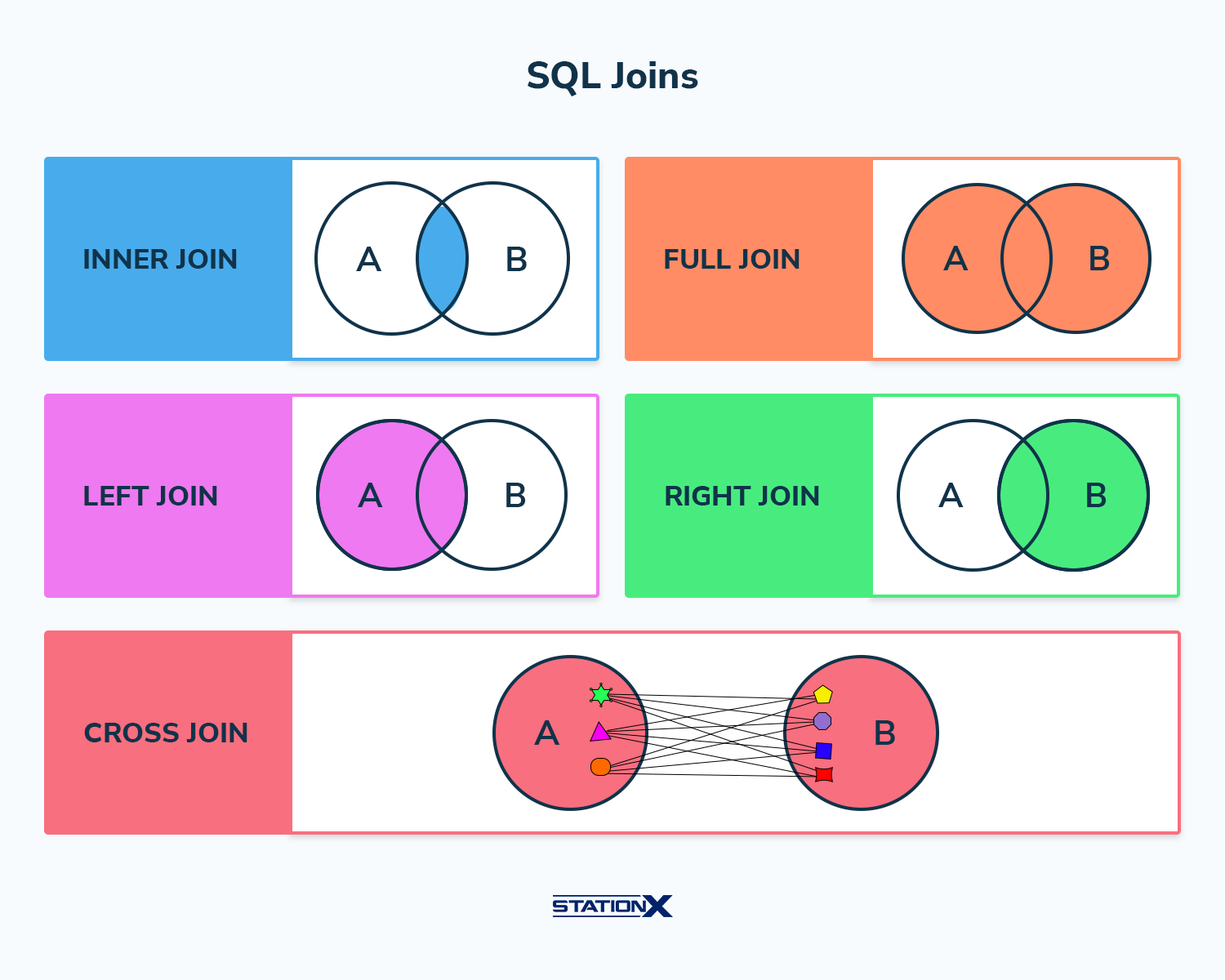
Sql joins
Temp Table (Temporary Table)
- Temp tables are created in the runtime and these tables are physically created in the tempdb database.
- Temp tables are similar to normal tables and also have constraints, keys, indexes, etc. We can perform all operations in the temp table like a normal table.
- The name of the temp table can have a maximum of 116 characters.
- The structure of temp table can be altered after creating it.
- There are below types of temp tables
- Local Temp Table
- Global Temp Table
Local Temp Table
- Local temp tables are only available to the current session that created them. The local temp tables are automatically deleted when the session is closed.
- Example: Let’s consider we are creating the temp table using query window. The temp table will only be available till query window is opened. If you close the current query window, then the temp table will be deleted. We can’t access that temp table with a new query window, it will throw the error.
- If the session that we are working on has subsequent nested sessions then, the temp tables will be visible in the nested sessions.
- The local temp table name is started with a single hash (“#”).
create table #Student
(
    Id int,
    Name nvarchar(50),
    Address nvarchar(150)
)
go
insert into #Student values ( 1, 'Test','Tamil Nadu');
go
select * from #Student;
When to use Local Temp Table?
- If the size of the temporary data is huge (more than 100 rows).
- When the user or connection which creates them alone can use it.
- If you need to create indexes or apply read lock, then go to temp table.
- You cannot use temp tables in User Defined Functions (UDF).
Global Temp Table
- Global temporary tables are temporary tables that are available for all sessions and all users. These can be created by any SQL Server connection user and these tables are automatically deleted when all the SQL Server connections are closed.
- The global temp table name is started with double hash (“##”).
create table ##Student
(
    Id int,
    Name nvarchar(50),
    Address nvarchar(150)
)
go
insert into ##Student values ( 1, 'Test','Tamil Nadu');
go
select * from ##Student;
When to use Global Temp Table?
- The global temp table has the same advantages over the local temp table with the feature of multiple users or sessions or connections should access to the same table.
Temp Variable
- Temp variable is similar to temp table to use holding the data temporarily.
- Table variable is a special kind of data type and is used to store the result set.
- The scope of temp variable is limited to the current batch and current Stored Procedure. It will delete once comes out the batch (Ex. Stored Procedure).
- We can create a primary key, identity in the temp variable.
- We cannot create non-clustered index. It can only have indexes that are automatically created with PRIMARY KEY and UNIQUE constraints as part of the creation.
- Temp Variable is also created in the tempdb database but not the memory.
- The Temp variable name is started with ”@”.
- Temp Variables are created using a “DECLARE” statement.
- We can use “insert into” statement for temp variable to store the values (Refer above examples)
- We cannot use “Select * into” statement for temp variable to store the values. First, we have to create a temp variable and insert the values into it.
- The name of the temp variable can have a maximum of 128 characters.
- Table variables can be passed as a parameter to functions and stored procedures.
Declare @My_var2 TABLE
(
   IID int,
   Name Nvarchar(50),
   Salary Int ,
   City_Name Nvarchar(50)
)

Insert Into @My_var2
Select * from Employee

Update @My_var2 Set name='Pankaj Kumar Choudhary'
where IID >2

Delete From @My_var2 Where IID=1
Select * from @My_var2
When to use Table Variable?
- To store the temporary data in user-defined functions (UDF), stored procedures, and query batches.
- If the volume of data is less, say less than 100 rows.
- If you don’t want to alter the table structure after creating it.
CTE (Common Table Expression)
- It is used to hold the temporary result set or result of complex sub-query.
- The scope of CTE is _limited to the current quer_y.
- CTE improves readability and ease in the maintenance of complex queries and sub-queries.
- CTE is created by using “WITH” statement and begin with a semicolon (;).
- There are two types of Common Table Expression
- Non-Recursive CTE - It does not have any reference to itself in the CTE definition.
- Recursive CTE - When a CTE has reference in itself, then it’s called recursive CTE.
SELECT id,total
FROM orders
WHERE
-- filter for orders with above-average totals (total is the CTE)
total > (
    SELECT
    AVG(total)
    FROM
    orders
)
When to use CTE?
- This is used to store the result of a complex subquery for further use.
- This is also used to create a recursive query.
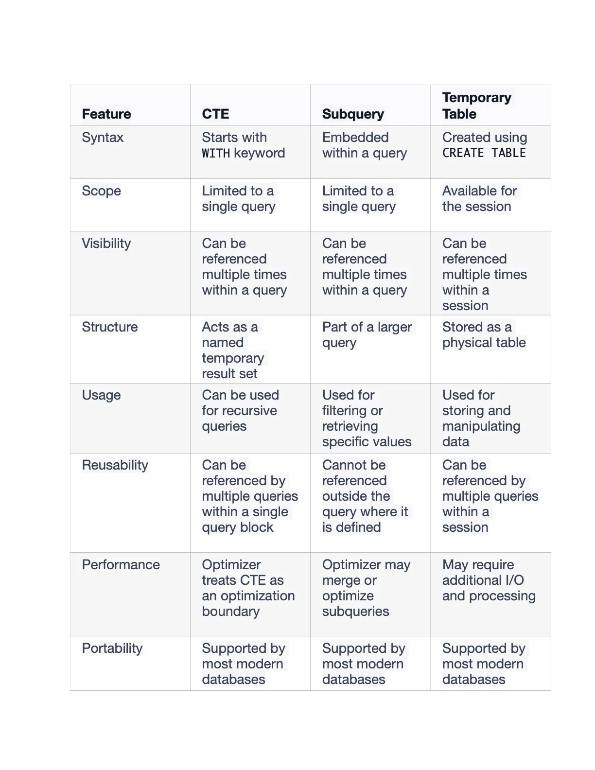
cte vs subquery vs temp table
SQL indexes
- An index can be created in a table to find data more quickly and efficiently.
- Index is a data structure (most commonly a B- tree) that stores the values for a specific column in a table.
- B- trees are more commonly used because the data that is stored inside the B- tree can be sorted.
- When we are looking for exact value (clustered value) from table then it searches for that record.
- If we are looking for some more values like in between, less than or greater than then it will not be beneficial because when we search any single value then its directly point to row data in a table.
- Indexes with appropriate column work like an array where value is directly searched into a column. For example, if we search for the following record:
select * from library where Book_Name = 'CsharpCorner_Book490000' - Then we are looking for ‘CsharpCorner_Book490000’. This values is in our table and hence our CPU time gets divided by using Index applied on it.
Physical operator on indexes
Physical operator is an object or routine that performs an operation like Index Delete, Index Insert, Index Scan, Index Seek etc
CREATE INDEX idx_lastname
ON Persons (LastName);
For more deatils on indexes and details
sql views
A view is a ‘virtual table’ containing fields from one or more tables.
A view is a logical view on one or more tables. A view on one or more tables i.e, the data from a view is not actually physically stored instead being derived from one or more tables. A view can be used to summarize data which is distributed among several tables
You can think of a view as a virtual table environment that’s created from one or more tables so that it’s easier to work with data.
A view is a virtual table. Every view has a Query attached to it. (The Query is a SELECT statement that identifies the columns and rows of the table(s) the view uses.)
CREATE VIEW us_customers AS
SELECT customer_id, first_name
FROM Customers
WHERE Country = 'USA';
Types of View in sql
Simple View: A view based on only a single table, which doesn’t contain GROUP BY clause and any functions.
CREATE VIEW V_Customer
AS SELECT First_Name, Last_Name, Country
FROM Customer;
Complex View: A view based on multiple tables, which contain GROUP BY clause and functions.
Inline View: A view based on a subquery in FROM Clause, that subquery creates a temporary table and simplifies the complex query.
Materialized View: A view that stores the definition as well as data. It creates replicas of data by storing it physically.
CREATE MATERIALIZED VIEW user_purchase_summary AS SELECT
  u.id as user_id,
  COUNT(*) as total_purchases,
  SUM(CASE when p.status = 'cancelled' THEN 1 ELSE 0 END) as cancelled_purchases
FROM users u
JOIN purchases p ON p.user_id = u.id;
sql projections
A projection is a value that is returned by a query statement (SELECT, MATCH).
Eg. the following query
SELECT name as firstName, age * 12 as ageInMonths, out("Friend") from Person where surname = 'Smith'
has three projections:
- name as firstName
- age * 12 as ageInMonths
- out(“Friend”)
partions
Database partitioning (also called data partitioning) refers to breaking the data in an application’s database into separate pieces, or partitions. These partitions can then be stored, accessed, and managed separately.
Types of database partitioning
Vertical partitioning
Vertical partitioning is when the table is split by columns, with different columns stored on different partitions.
In vertical partitioning, we might split the table above up into two partitions, one with the id, username, and city columns, and one with the id and balance columns.
Horizontal partitioning
Horizontal partitioning is when the table is split by rows, with different ranges of rows stored on different partitions.
To horizontally partition our example table, we might place the first 500 rows on the first partition and the rest of the rows on the second
Partition algorithms
- RANGE partitioning. This type of partitioning assigns rows to partitions based on column values falling within a given range.
CREATE TABLE employees (
    id INT NOT NULL,
    fname VARCHAR(30),
    lname VARCHAR(30),
    hired DATE NOT NULL DEFAULT '1970-01-01',
    separated DATE NOT NULL DEFAULT '9999-12-31',
    job_code INT NOT NULL,
    store_id INT NOT NULL
)
PARTITION BY RANGE (store_id) (
    PARTITION p0 VALUES LESS THAN (6),
    PARTITION p1 VALUES LESS THAN (11),
    PARTITION p2 VALUES LESS THAN (16),
    PARTITION p3 VALUES LESS THAN MAXVALUE
);
LIST partitioning. Similar to partitioning by RANGE, except that the partition is selected based on columns matching one of a set of discrete values.
CREATE TABLE employees (
    id INT NOT NULL,
    fname VARCHAR(30),
    lname VARCHAR(30),
    hired DATE NOT NULL DEFAULT '1970-01-01',
    separated DATE NOT NULL DEFAULT '9999-12-31',
    job_code INT,
    store_id INT
)
PARTITION BY LIST(store_id) (
    PARTITION pNorth VALUES IN (3,5,6,9,17),
    PARTITION pEast VALUES IN (1,2,10,11,19,20),
    PARTITION pWest VALUES IN (4,12,13,14,18),
    PARTITION pCentral VALUES IN (7,8,15,16)
);
HASH partitioning. With this type of partitioning, a partition is selected based on the value returned by a user-defined expression that operates on column values in rows to be inserted into the table. The function may consist of any expression valid in MySQL that yields an integer value.
CREATE TABLE employees (
    id INT NOT NULL,
    fname VARCHAR(30),
    lname VARCHAR(30),
    hired DATE NOT NULL DEFAULT '1970-01-01',
    separated DATE NOT NULL DEFAULT '9999-12-31',
    job_code INT,
    store_id INT
)
PARTITION BY HASH( YEAR(hired) )
PARTITIONS 4;
CREATE TABLE employees (
    id INT NOT NULL,
    fname VARCHAR(30),
    lname VARCHAR(30),
    hired DATE NOT NULL DEFAULT '1970-01-01',
    separated DATE NOT NULL DEFAULT '9999-12-31',
    job_code INT,
    store_id INT
)
PARTITION BY LINEAR HASH( YEAR(hired) )
PARTITIONS 4;
KEY partitioning. This type of partitioning is similar to partitioning by HASH, except that only one or more columns to be evaluated are supplied, and the MySQL server provides its own hashing function. These columns can contain other than integer values, since the hashing function supplied by MySQL guarantees an integer result regardless of the column data type.
CREATE TABLE k1 (
    id INT NOT NULL,
    name VARCHAR(20),
    UNIQUE KEY (id)
)
PARTITION BY KEY()
PARTITIONS 2;
sharding
Sharding refers to splitting the data in one database and storing them in multiple tables and databases according to some certain standard, so that the performance and availability can be improved. Both methods can effectively avoid the query limitation caused by data exceeding affordable threshold. What’s more, database sharding can also effectively disperse TPS. Table sharding, though cannot ease the database pressure, can provide possibilities to transfer distributed transactions to local transactions, since cross-database upgrades are once involved, distributed transactions can turn pretty tricky sometimes. The use of multiple primary-replica sharding method can effectively avoid the data concentrating on one node and increase the architecture availability.
Splitting data through database sharding and table sharding is an effective method to deal with high TPS and mass amount data system, because it can keep the data amount lower than the threshold and evacuate the traffic. Sharding method can be divided into vertical sharding and horizontal sharding.
Vertical Sharding
According to business sharding method, it is called vertical sharding, or longitudinal sharding, the core concept of which is to specialize databases for different uses. Before sharding, a database consists of many tables corresponding to different businesses. But after sharding, tables are categorized into different databases according to business, and the pressure is also separated into different databases. The diagram below has presented the solution to assign user tables and order tables to different databases by vertical sharding according to business need.
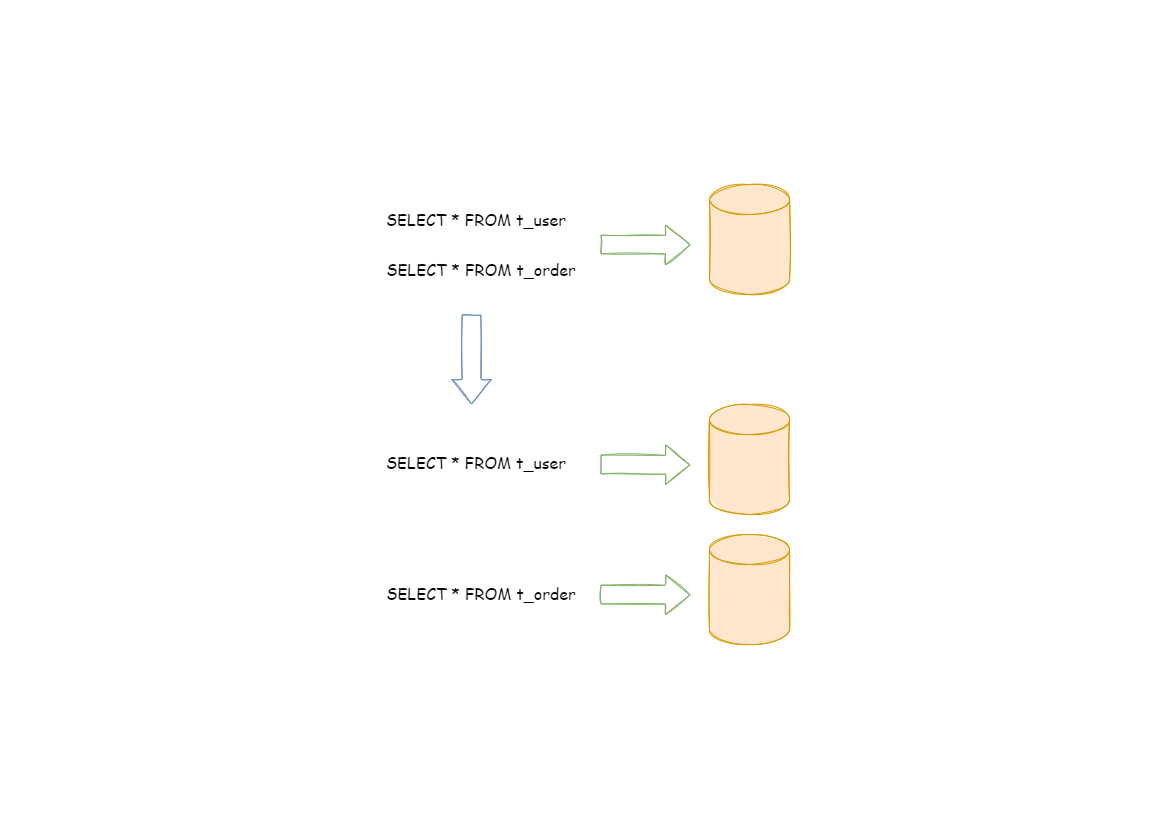
Vertical sharding requires to adjust the architecture and design from time to time. Generally speaking, it is not soon enough to deal with fast changing needs from Internet business and not able to really solve the single-node problem. it can ease problems brought by the high data amount and concurrency amount, but cannot solve them completely. After vertical sharding, if the data amount in the table still exceeds the single node threshold, it should be further processed by horizontal sharding.
Horizontal Sharding
Horizontal sharding is also called transverse sharding. Compared with the categorization method according to business logic of vertical sharding, horizontal sharding categorizes data to multiple databases or tables according to some certain rules through certain fields, with each sharding containing only part of the data. For example, according to primary key sharding, even primary keys are put into the 0 database (or table) and odd primary keys are put into the 1 database (or table), which is illustrated as the following diagram.
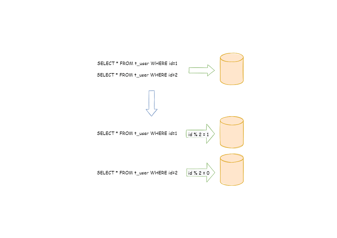
Theoretically, horizontal sharding has overcome the limitation of data processing volume in single machine and can be extended relatively freely, so it can be taken as a standard solution to database sharding and table sharding.
Storage engines
Storage engines are MySQL components that handle the SQL operations for different table types. InnoDB is the default and most general-purpose storage engine, and Oracle recommends using it for tables except for specialized use cases. (The CREATE TABLE statement in MySQL 8.0 creates InnoDB tables by default.)
-
InnoDB: The default storage engine in MySQL 8.0. InnoDB is a transaction-safe (ACID compliant) storage engine for MySQL that has commit, rollback, and crash-recovery capabilities to protect user data. InnoDB row-level locking (without escalation to coarser granularity locks) and Oracle-style consistent nonlocking reads increase multi-user concurrency and performance. InnoDB stores user data in clustered indexes to reduce I/O for common queries based on primary keys. To maintain data integrity, InnoDB also supports FOREIGN KEY referential-integrity constraints. For more information about InnoDB, see Chapter 15, The InnoDB Storage Engine.
-
MyISAM: These tables have a small footprint. Table-level locking limits the performance in read/write workloads, so it is often used in read-only or read-mostly workloads in Web and data warehousing configurations.
-
Memory: Stores all data in RAM, for fast access in environments that require quick lookups of non-critical data. This engine was formerly known as the HEAP engine. Its use cases are decreasing; InnoDB with its buffer pool memory area provides a general-purpose and durable way to keep most or all data in memory, and NDBCLUSTER provides fast key-value lookups for huge distributed data sets.
-
CSV: Its tables are really text files with comma-separated values. CSV tables let you import or dump data in CSV format, to exchange data with scripts and applications that read and write that same format. Because CSV tables are not indexed, you typically keep the data in InnoDB tables during normal operation, and only use CSV tables during the import or export stage.
-
Archive: These compact, unindexed tables are intended for storing and retrieving large amounts of seldom-referenced historical, archived, or security audit information.
-
Blackhole: The Blackhole storage engine accepts but does not store data, similar to the Unix /dev/null device. Queries always return an empty set. These tables can be used in replication configurations where DML statements are sent to replica servers, but the source server does not keep its own copy of the data.
-
NDB (also known as NDBCLUSTER): This clustered database engine is particularly suited for applications that require the highest possible degree of uptime and availability.
-
Merge: Enables a MySQL DBA or developer to logically group a series of identical MyISAM tables and reference them as one object. Good for VLDB environments such as data warehousing.
-
Federated: Offers the ability to link separate MySQL servers to create one logical database from many physical servers. Very good for distributed or data mart environments.
-
Example: This engine serves as an example in the MySQL source code that illustrates how to begin writing new storage engines. It is primarily of interest to developers. The storage engine is a “stub” that does nothing. You can create tables with this engine, but no data can be stored in them or retrieved from them.
Data Replication
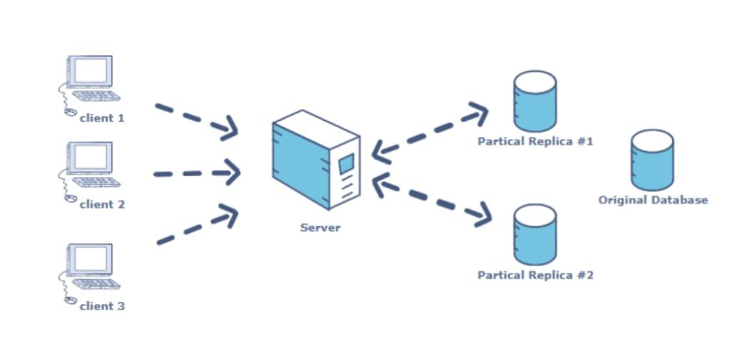
Data replication refers to the process of generating numerous copies of complex datasets and storing them across various locations to facilitate seamless access. It plays a crucial role in ensuring the high availability of data for individual systems and numerous servers. Data replication uses two types of storage locations, namely master and snapshot storage areas. Data replication follows the same concept as copying data from one database to another; however, it allows all the users to access the same data seamlessly and without any inconsistencies.
Understanding the Need & Benefits of Setting up Replication
Having only one copy of your crucial business data can be risky for any organization worldwide, as it can result in a loss of credibility and potential business opportunities. Such issues can arise when there is an unpredictable or untimely server malfunction, database hacks, loss of data, and many other technical faults, resulting in the data associated with your business process becoming unavailable.
Setting up data replication and maintaining multiple copies of your business data across servers, devices, etc., is a robust way to tackle such risks and ensure high data availability at all times.
Key Benefits of Setting up Data Replication
- Data replication allows users spread across diverse geographies, to access data seamlessly by letting them access the replica closest to them.
- It helps reduce costs associated with bandwidth and maintenance.
- It boosts data throughput and provides a robust disaster recovery mechanism.
- It helps set up effective analytics and business intelligence-based processes.
Data Replication Strategies
Some of the most popular and robust data replication strategies that you can use to start replicating your data are as follows. They are divided into two kinds: incremental data replication, and full table data replication.
Incremental Data Replication

1. Log-based Incremental Data Replication
Most database-based solutions keep track of every change in the database, right from the very beginning. It further generates a record for the same, known as a log file or changelog. Each log file acts as a collection of log messages, each containing data such as the time/user/change/cascade effects/method of the change. The database then assigns a unique position Id to all of them and stores them in an Id-based chronological order.
You can implement log-based data replication in the following two ways:
Statement-Based Replication
Statement-based replication keeps track and stores all such commands, queries or actions that modify the database and bring about updations. Procedures that have the statement-based mechanism in place generate the replicas by re-running all these statements in the order of their occurrence.
Advantages of Statement-Based Replication
- The size of the log file generated in this technique is small. Replicas perform numerous cascading-based changes by making use of integrity constraints.
- It allows users to audit with ease.
Disadvantages of Statement-Based Replication
- Statement-based replication doesn’t allow replicating every command and its effects.
- Sometimes, executing commands or queries that have dependency constraints can result in numerous errors or data-related discrepancies.
- In case the replica’s hardware/operating system is not in the same state as the original database, statement execution can lead to undesirable results.
Row-Based Replication
Row-based replication keeps track of all the new rows of the database and stores them in the form of a record in the log file. Procedures that have a row-based replication mechanism in place carry out replication by iterating over each log message in the initial order of execution. Here, the position Id acts as a bookmark, allowing the database to easily continue the replication process.
Advantages of Row-Based Replication
- Row-based replication is one of the most accurate and safe strategies for carrying out data replication, as it ensures that the new rows replicate as per the log.
Disadvantages of Row-Based Replication
- SQL statements often bring about changes across numerous rows and tables, so the log file will have to store all these files.
- The mechanism of row-based replication is time and resource-consuming.
- Log files take up a lot of memory or space, in case the columns that you update are of the BLOB or MIME type.
- If a log remains locked for writes, then the replication or the “read” process will have to wait for a significant amount of time.
2. Key-based Incremental Data Replication
Modern databases across all organizations receive and generate updates nearly in real-time or very frequently, which can contain a diverse data set such as text, audio, videos, etc. Databases then chain such updates with the ones that happen shortly afterward, often generated by a diverse set of sources or actors. If your database has varied data requirements, focuses more on the new data updates rather than historical values, and further stores data records based on unique Ids/keys, then “key-based incremental replication” is the right choice.
Key-based incremental data replication leverages the replication key column to identify the new and updated data. It then carries out the replication process for records that house the updated replication keys. Hence, only these rows undergo any updates, with their previous key values getting either erased or overwritten. It thus maintains the latest values associated with these keys.
Numerous enterprise-grade databases, such as PostgreSQL, Oracle, Salesforce, etc., use key-based incremental strategy to replicate data with ease.
Advantages of Key-Based Incremental Data Replication
- Key-based incremental data replication focuses only on new and modified data and hence, requires less bandwidth & compute resources to carry out replication in a quick manner.
Disadvantages of Key-Based Incremental Data Replication
- Key-based incremental data replication automatically deletes the replication key associated with a record in case the data record gets deleted.
- Keeping track or tracing back the historical values of the new data records can be challenging as this technique doesn’t maintain a change history.
Full Table Data Replication Strategy
Full table Data Replication Strategy focuses on replicating the database and its table completely. It will replicate all the data records, regardless of whether they are old or new. This mechanism can come in handy when you’re replicating data across old and new tables with no definition-based difference or when the data rows don’t have primary keys associated with them. Small databases such as website CDNs have this mechanism in place.
Modern databases implement full table replication using either of the following two variations of this technique:
1. Snapshot Replication

Snapshot Replication in MS SQL
Snapshot replication generates a replica of your database by taking a “snapshot” of how your tables, data, relationships, etc., look like at a particular point in time and then replicates the same on the other database. It only captures this snapshot when it needs to copy the data; hence, it does not monitor any updates. It is suitable for databases where updates aren’t frequent, for example, insurance agents, sales, etc. Various popular databases implement this technique to carry out data replication.
2. Transactional Replication

Transaction Replication in MS SQL
Transactional replication achieves replication by first monitoring the updates as they occur on the master database and then carrying out sync to make all these changes in the replicas. It ensures transactional consistency by carrying out the updates in the same order as the original database. Transactional replication can be a fruitful technique to meet business intelligence and analytics-related business requirements, focusing more on historical data rather than current data. Microsoft SQL Server is one such enterprise-grade database that implements this technique.
Advantages of Full Table Data Replication
- It is one of the most robust strategies that ensure that the replicas are an exact mirror image of the original table.
- It helps create exact replicas across different geographies, which results in faster queries and good throughput time.
Disadvantages of Full Table Data Replication
- It requires a lot of bandwidth related to processing power, resources, etc., as it operates by creating a full copy in each replication attempt.
- Replicating the entire database can be cumbersome, often resulting in numerous errors.
levels of isolation
Certainly! Below is an expanded explanation of isolation levels in RDBMS with examples, tradeoffs, and Mermaid scripts to illustrate the concepts visually.
Isolation Levels in RDBMS
Isolation levels in RDBMS determine how transactions interact with each other and the level of data consistency and integrity maintained during concurrent transactions. They play a crucial role in maintaining the ACID properties (Atomicity, Consistency, Isolation, Durability) of transactions.
Isolation Level Examples
Let’s consider each isolation level with an example:
Read Uncommitted:
Example:
Read Committed:
Example:
Repeatable Read:
Example:
Serializable:
Example:
Tradeoffs
The tradeoffs associated with each isolation level are as follows:
$ Read Uncommitted$: Allows for dirty reads, sacrificing data consistency for high concurrency.
$ Read Committed$: Prevents dirty reads but allows non-repeatable reads and phantom reads, balancing concurrency and consistency.
$ Repeatable Read$: Ensures a consistent snapshot of data, preventing dirty reads, non-repeatable reads, and phantom reads, but may allow for potential write skew anomalies.
$ Serializable$ : Provides the highest level of data consistency but can lead to increased contention and reduced concurrency due to the need for locks.
Sure, here’s the information in markdown format:
Issues with Isolation Levels in RDBMS
Some of the common issues and challenges associated with isolation levels in RDBMS include:
$ Concurrency Control Overhead$ : Higher isolation levels often require more extensive locking or versioning mechanisms to maintain data consistency, which can introduce overhead and reduce concurrency.
$ Phantom Reads$ : In non-serializable isolation levels, phantom reads can occur, where a transaction retrieves a set of records that satisfy a search condition and a second transaction inserts new records that match the condition, causing the first transaction to re-run and retrieve a different set of records.
$ Non-Repeatable Reads$ : At lower isolation levels, non-repeatable reads can occur, where a transaction retrieves a record, another transaction modifies or deletes the record, and the first transaction retrieves the same record again, obtaining different results.
$ Write Skew Anomalies$ : In multi-version concurrency control, write skew occurs when two transactions read an overlapping set of data and update it independently, leading to inconsistent results.
$ Deadlocks$ : Stricter isolation levels can increase the likelihood of deadlocks where two or more transactions are unable to proceed because each is waiting for the other to release a lock.
$ Reduced Concurrency$ : Higher isolation levels may lead to reduced concurrency and increased contention due to the need for more restrictive locking or validation mechanisms.
$ Performance Impact$ : More stringent isolation levels can impact the overall performance of the database due to increased locking, reduced parallelism, and additional checks for data consistency.
$ Complexity and Maintenance$ : Managing and tuning isolation levels, especially in a complex application with numerous concurrent transactions, can be challenging and require ongoing maintenance and optimization.
Understanding these issues is crucial for database administrators and application developers to select the appropriate isolation level that balances data consistency and concurrency while mitigating potential challenges.